Abstract

Steepest ascent/descent and stochastic gradient ascent/descent are widely used techniques to approximate parameters for multiple linear regression, logistic regression, and artificial neural networks to name a few. However, one of the problems with stochastic gradient ascent/descent is that in most cases it does not converge and rather wanders around the approximate solution. To get convergence, we parallelized (multithreaded) stochastic gradient ascent for logistic regression and took the average of the updated parameters from each thread. This average updated parameter was then used in the next iteration of the stochastic gradient approach. This not only speeds up the calculation but also is an effective way to get convergence for stochastic gradient approaches. Wine data for the Quality was used to analyze and justify this approach.

Introduction

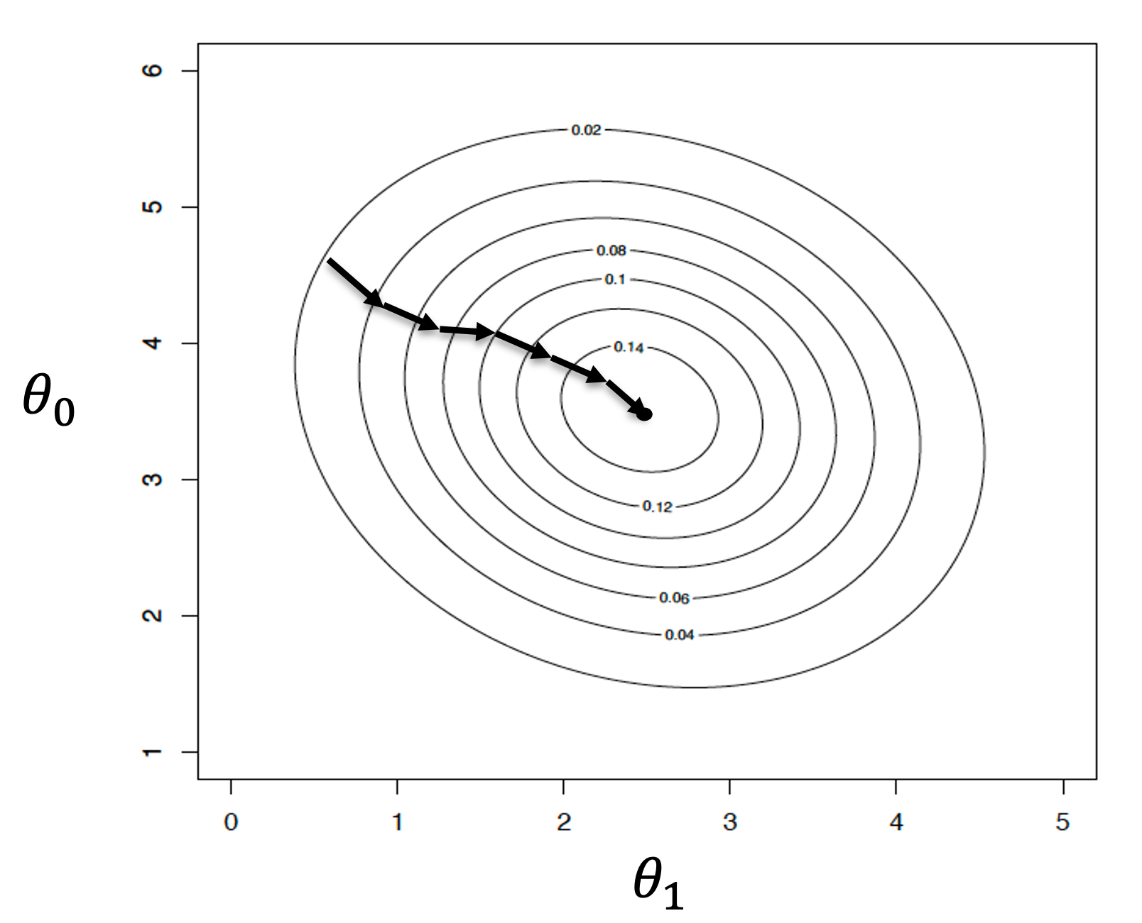
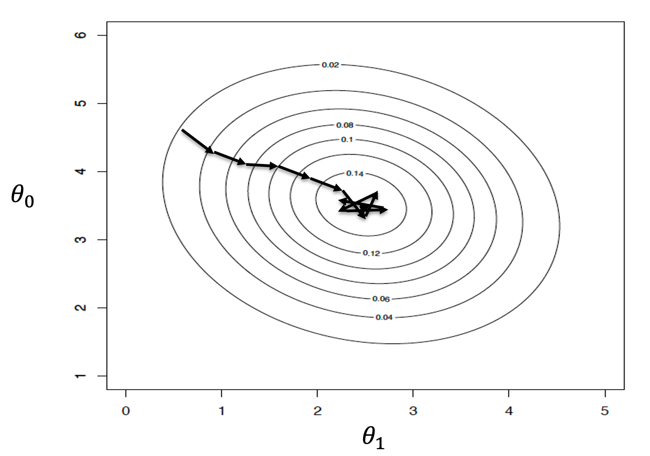
Stochastic steepest gradient ascent (SGA) is a well know numerical method which is used to solve logistic regression. However, one of the problems with this method is that it bounces around the solution and may times never converges to the approximate solution for a good initial guess. On the other hand, the standard steepest gradient ascent will converge smoothly to the approximate solution with a good initial guess. This convergence behavior is show below for a simple logistic model with only parameters.

Hypothesis

For this study we prdopose a parallelized version of stochastic steepest gradient ascent (SGA) for logistic regression, where batches are divided among multiple threads, and the parameter updates are synchronized periodically. We conduct a series of experiments on various datasets and benchmark the parallelized stochastic SGA against the standard SGA implementation. Our results demonstrate that the parallelized approach significantly reduces the execution time while maintaining similar convergence behavior to SGA. Furthermore, we analyze the impact of different thread configurations and mini-batch sizes on the convergence performance. These findings provide valuable insights for researchers and practitioners seeking to accelerate the training process of machine learning models using parallel computing techniques.

Gradient Ascent

Gradient Ascent is an iterative algorithm used for optimizing the error squared between the proposed functions (proposed parameters for the function) outputs and the actual outputs. The general cost function and error function is as shown.

import numpy as np
 
    def gradient(self, X, y, theta):
        m = len(y)
        h = self.logit(np.dot(X, theta))
        grad = (1 / m) * np.dot(X.T, (h - y))
        return grad

Cost Function

where 𝑚 is the number of rows, $\vec{x}^{(i)}$ is the vector of input data for row i, $y_i$ is the output for row i while $h(\vec{x}^{(i)}, \vec{\theta})$ is the function we are trying to fit to the data. The gradient of this cost function for logistic regression is well know and can be generalized as

1. \ \frac{\partial J}{\partial \theta_k} = \sum_{i=0}^m \left( (h(\theta^T \cdot x^{(i)}) - y_i) \cdot x_k^{(i)} \right)

import numpy as np
 
   def cost_function(self, X, y, theta):
       m = len(y)
       h = self.logit(np.dot(X, theta))
       y_array = np.array(y)  # Convert list to numpy array
       epsilon = 1e-7  # Small constant to prevent log(0)
       cost = (-1 / m) * np.sum(y_array.reshape(-1, 1) * np.log(h +
                                                                epsilon) + (1 - y_array.reshape(-1, 1)) * np.log(1 - h + epsilon))
       return cost

Where k is the kth parameter and for k=1 a column of ones was added to utilize the dot product in our calculations. The iterative scheme for stochastic gradient ascent is shown below

Iterative Shceme For Gradient Ascent

2. \ \begin{bmatrix} \theta_0^n \\ \theta_1^n \\ \theta_2^n \end{bmatrix} = \begin{bmatrix} \theta_0^{n-1} \\ \theta_1^{n-1} \\ \theta_2^{n-1} \end{bmatrix} + \alpha \nabla J(\theta)

For stochastic gradient ascent instead of running of the sum in equation (2) we update the parameters each time a row of data is used or consider various rows of data (batches) to update the parameters.

Parallelization

Multi-core CPUs and can lead to near-linear speed-ups relative to the number of available cores. However, it's important to manage inter-process communication and synchronization

Mini-Batches

Processing of mini-batches in Stochastic Gradient Ascent (SGA) can significantly accelerate training times for large datasets. By distributing mini-batches across multiple processors, each processor can independently compute the gradient and update the model parameters.

 
from multiprocessing import Pool
 
    num_ranks = 10
    processes = []
 
    # Calculate the size of each mini-batch
    mini_batch_size = len(StochasticGradient().target) // num_ranks
 
    # Create a list of arguments for each mini-batch
    args_list = []
    for i in range(num_ranks):
        data = StochasticGradient()
        start = i * mini_batch_size
        end = (i + 1) * mini_batch_size if i < num_ranks - \
            1 else len(data.target)
        args_list.append((data, start, end, 1000, mini_batch_size))
 
    # Use a process pool to process each mini-batch in parallel
    with Pool(num_ranks) as pool:
        results = pool.map(run_sgd, args_list)

Results

Conclusion

GitHub release (latest SemVer)